paper review - Llama 3 Herd of Models

_{scroll ↓ to Resources}

Abstract

This paper presents a new set of foundation models, called Llama 3. It is a herd of language models that natively support multilinguality, coding, reasoning, and tool usage. Our largest model is a dense Transformer with 405B parameters and a context window of up to 128K tokens.
Llama 3 delivers comparable quality to leading language models such as GPT-4 on a plethora of tasks.

Introduction

three key levers in the development of high-quality foundation models: data, scale and managing complexity

We pre-train Llama 3 on a corpus of about 15T multilingual tokens, compared to 1.8T tokens for Llama 2

While our scaling laws suggest our flagship model is an approximately compute-optimal size for our training budget, we also train our smaller models for much longer than is compute-optimal. The resulting models perform better than compute-optimal models at the same inference budget. We use the flagship model to further improve the quality of those smaller models during post-training

this is over-training - using more compute power for pre-training smaller (8B) models, than they optimally require according to scaling laws for given model size. E

We make design choices that seek to maximize our ability to scale the model development process. For example, we opt for a standard dense transformer model architecture (Vaswani et al., 2017) with minor adaptations, rather than for a mixture-of-experts model (Shazeer et al., 2017) to maximize training stability. …

preference for conservative, but controllable choices, which ensures less complications during training. This includes some hardware choices (there is a separate chapter about that), but also e.g. choice for direct preference optimization instead of RLHF, which is less stable and more complex to scale.

General overview

architecture: classic dense decoder-only transformer (not mixture-of-experts) from Attention Is All You Need
- see below for 3.2 Model architecture
development comprises from model Pre-training and Post-training

Pre-training

See 3 Pre-training below for details
Goal: next token prediction on a large corpus, not instruction following

the model learns the structure of language and obtains large amounts of knowledge about the world from the text it is “reading”.

To do this effectively, pre-training is performed at massive scale: we pre-train a model with 405B parameters on 15.6T tokens using a context window of 8K tokens. This standard pre-training stage is followed by a continued pre-training stage that increases the supported context window to 128K tokens.

First they train on a small context window (8K), then increase it to 128K tokens. Reasoning: remember that the attention mechanism is quadratic in memory-complexity. Combine that with the assumption that in the beginning there is no big win for the model to have huge context. Later on, switch to 128K context is beneficial so that the model can learn to look far away. Implementation wise, in the first stage they had input longer than 8K too, but forbid the model to look beyond this limit. This can be done using masked MHA, but we don’t know if they did exactly that.

Multi-modal adapter (vision, speech) pre-training: out of the scope of this review for now

Post-training

See 4 Post-training below for details
any model training that happens outside of the pre-training - teach the model to follow instructions, behave as an assistant; integrate tools usage for coding, reasoning; incorporate safety mitigations.

3 Pre-training

3.1 Pre-training data preprocessing

data quality

preprocessing steps

deduplication: many duplicates of the same text may lead to the model assigning one token for long sequences

url-level, document-level and line-level deduplication

heuristic filtering

removing duplicated lines which are different: logging, error messages

dirty words counting

Kullback-Leibler divergence to filter out documents with many outliers comparing to the training corpus token distribution

model-based quality filtering: find high-quality tokens

light text classifiers as fasttext

heavy pipelines: ^a7b252

use high performing LLM (Llama 2) to label a training dataset (define if documents meet given quality requirements)

train a simpler BERT-based classifier (Roberta) using labels made by Llama 2

use new Roberta model to classify the large text corpus for Llama 3.

code and reasoning data

HTML parsers, preserving math and code structure

pipeline similar to above, but with prompt tuning to account for the data type

multi-lingual data

similar approach as for English, but for each language

quality-ranking and balancing amount of tokens per language to optimize for English and multilingual benchmarks

general cleaning, remove personally identifiable info, adult content

remove markdown as its presence has shown to deteriorate the results

3.1.2 Determining the data mix

knowledge classification: categorize data into categories (e.g. arts, entertainment) and downsample over-represented ones
scaling laws for data mix: train several small models and use those to predict performance of a large model on that mix. Try several data mixes and choose the most promising.
- ==scaling laws is one of the main instruments for training LLM in a data-driven way==

Our final data mix contains roughly 50% of tokens corresponding to general knowledge, 25% of mathematical and reasoning tokens, 17% code tokens, and 8% multilingual tokens

3.1.3 Annealing data

Research shows that using your best quality (or domain-specific) data in the latest stage of training, has huge positive effect. Or, in other words, tokens in the end of training have disproportionally high impact on model quality

We find that annealing improved the performance of a pre-trained Llama 3 8B model on the GSM8k and MATH validation sets by 24.0% and 6.4%, respectively. However, the improvements on the 405B model are negligible, suggesting that our flagship model has strong in-context learning and reasoning capabilities and does not require specific in-domain training samples to obtain strong performance.

Annealing to asses data quality

one of the methods of learning rate decay is constant and then linear decay. It has been shown that there is training boost during the decay part
they took a 50% trained (probably % refers to the total number of tokens) small 8B-parameters model and anneal learning rate linearly to 0 while continue training on a mix of the default data mix (70%) and a new dataset (30%), which quality they want to evaluate. Total number of tokens in this mix is 40B, which is very few comparing to the whole corpus of 1.5T. This is computationally affordable and can be repeated on a number of datasets. Final model performance is indicative of dataset quality. This method works better than scaling laws

3.2 Model architecture

classic transformer (Attention Is All You Need) similar to Llama and Llama 2: Open Foundation and Fine-Tuned Chat Models
- Performance gains primarily due to data quality and diversity, as well as increased training scale.

Details

Contents

We adopt most of the pretraining setting and model architecture from Llama 1. We use the standard transformer architecture (Vaswani et al., 2017), apply pre-normalization using RMSNorm (Zhang and Sennrich, 2019), use the SwiGLU activation function (Shazeer, 2020), and rotary positional embeddings (RoPE, Su et al. 2022). The primary architectural differences from Llama 1 include increased context length and grouped-query attention (GQA).

Activation function SwiGLU, just because it works

compared to Llama 2:

grouped query attention already used in Llama 2, but now with less key-value heads for speed optimizationy

128K tokens vocabulary, compression rate 3.94 characters per token, 28K tokens specifically added to improve multilanguage performance

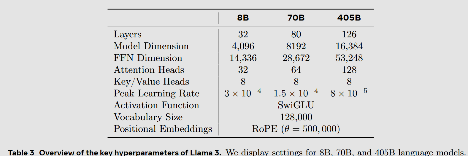
Llama 3 405B uses an architecture with 126 layers, a token representation dimension of 16,384, and 128 attention heads; see Table 3 for details. This leads to a model size that is approximately compute-optimal according to scaling laws on our data for our training budget of 3.8 × 1025 FLOPs.

3.2.1 scaling laws

Challenge

determine the optimal model size for given compute power and desired benchmarks - without actually training the model, because of the costs involved
- Existing scaling laws typically predict only next-token prediction loss rather than specific benchmark performance.
- Scaling laws can be noisy and unreliable because they are developed based on pre-training runs conducted with small compute budgets
essentially, we can’t predict final benchmark results from intermediate benchmark results. therefore, they first establish correlation between intermediate next-token-prediction results with final next-token-prediction results. Then they establish correlation between final next-token-prediction results and final benchmark results.

Methodology

scaling laws > Llama 3

3.4 Training Recipe

Similar for all three models with 8, 70, or 405 billion parameters.

3.4.1 Initial pre-training

learning rate decay doesn’t go to 0, but to a very small number $8 \times 1 0^{- 7}$

We use a lower batch size early in training to improve training stability, and increase it subsequently to improve efficiency. Specifically, we use an initial batch size of 4M tokens and sequences of length 4,096, and double these values to a batch size of 8M sequences of 8,192 tokens after pre-training 252M tokens. We double the batch size again to 16M after pre-training on 2.87T tokens.

it is general knowledge, that larger batch size improves gradient descent algorithm estimation. ==What is their gain in lowering it on initial learning?==

Adjusting the data-mix

3.4.2 Long context pre-training

Train the model on longer sequences than initially to teach the model to support longer context length up to 128K tokens. It is computationally expensive to use long sequences from the beginning. This increment is done in multiple steps, after each time they track how the model adapts to the new sequence length.
- Successful adaptation is measured by two factors:
  - Model performance on short context evaluations has recovered completely. Training the model on longer sequences may change model parameters and (temporary) negatively affect the performance of the model on shorter sequences.
  - the model perfectly solves “needle in a haystack” tasks up to that length.

3.4.3 Annealing

See also 3.1.3 Annealing data
TLDR: using high quality data is extremely beneficial during the last stage of pre-training.
The final pre-trained model is computed as the average of model checkpoints during annealing.
- Unlike in random forest they don’t average out the predictions (results), but rather average out model parameters (weights) directly.
- The average checkpoint will be better than the last one in terms of its ability to generalize.

4 Post-training

We produce the aligned Llama 3 models by applying several rounds of post-training, or aligning the model with human feedback on top of a pre-trained checkpoint. Each round of post-training involves supervised finetuning (SFT) followed by direct preference optimization (DPO) on examples collected either via human annotations or generated synthetically.

Pre-training goal was to model the language and predict the next token. Instruction following was not in the focus, this is what post-training is about.

Post-training approach illustration

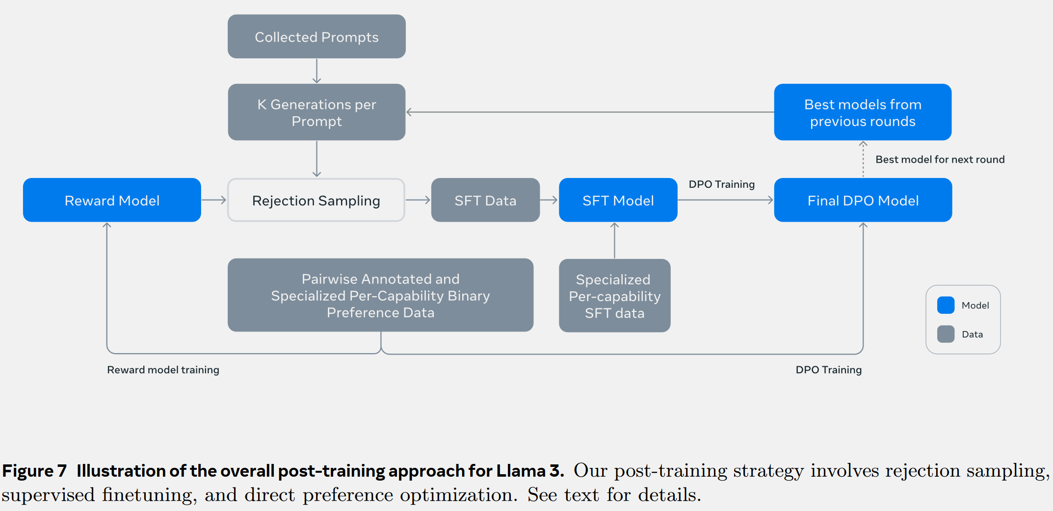
There are six cycles of this post-training procedure. Each includes rejection sampling, SFT and the DPO. Each new cycle uses the DPO model from the previous cycle. The first cycle uses a checkpoint after 3 Pre-training as the starting point.
First, 4.1.2 Reward modeling is created from pairwise-annotated data and current best model.
Reward model is used for Rejection sampling (filtering out and allow further only generated prompts with highest scores).
Filtered synthetic data in combination with Specialized per-capability SFT data (e.g. for coding, math, etc.) is used for SFT. The output SFT model is better.
SFT model is further optimized with DPO. This step doesn’t require the reward model, but only human preference data.
The DPO model become the best model, used for prompts generation for the next post-training cycle.

4.1. Modeling

Consists of several stages:
- Train a reward model on top of the pre-trained checkpoint using human-annotated preference data
- Fine-tune pre-trained checkpoints with supervised finetuning
- Align the checkpoints with direct preference optimization

4.1.1 Chat Dialog Format

LLama 3 enables tools usage and requires mode advanced chat dialog protocol allowing sending messages to different recepients (e.g. user, ipython). This is regulated by various headers and special tokens.

4.1.2 Reward modeling

authors used Bradley-Terry model as in Llama 2

see more in Note

Note

reward model is the result of training on top of the pre-trained LLM checkpoint

for any pair (instruction, result) predict a number (Reward Score) denoting how good is the result for this instruction - assigns a numerical score to model outputs based on their alignment with human preferences and values. The higher the score, the higher is the estimated degree of alignment.

use human-annotated data with several ranked responses for each given instruction, for instance: $e d i t e d > c h ose n > re j ec t e d$

in practice, there can be up to 9 ranked responses, some of which can be excluded if too hard to rank.

$e d i t e d$ response can be optionally added by human annotators to improve one of the existing responses

having such a model, we can select the best result from several options or use it for RLHF

Link to original

4.1.3 Supervized Finetuning

prior to supervised finetuning the 4.1.2 Reward modeling is used for rejection sampling to remove the worst pairs (instruction, result)
synthetic data is also part of the data mix
use the pre-trained checkpoint data
- reward model is ONLY used for rejection sampling and is not part of the checkpoint
see 4.2 Post-training Data

4.1.4 Direct Preference Optimization

Further improvement to make models align with human preferences.
some additions to the DPO:
- Masking out formatting (e.g. header and termination) tokens in DPO loss.

We mask out special formatting tokens including header
and termination tokens (described in Section 4.1.1) from both chosen and rejected responses in the
loss to stabilize DPO training. We observe that having these tokens contribute to the loss may lead
to undesired model behaviors such as tail repetition or abruptly generating termination tokens. We
hypothesize that this is due to the contrastive nature of the DPO loss – the presence of common tokens
in both chosen and rejected responses leads to a conflicting learning objective as the model needs to
increase and reduce the likelihood of these tokens simultaneously.

Regularization with an additional negative log-likelihood (NLL) loss

We add an additional negative log-likelihood (NLL) loss term with a scaling
coefficient of 0.2 on the chosen sequences, similar to Pang et al. (2024). This helps further stabilize DPO
training by maintaining desired formatting for generation and preventing the decrease of log probability
of chosen responses (Pang et al., 2024; Pal et al., 2024).

4.1.5 Model Averaging

Finally, we average models obtained from experiments using various versions of data or hyperparameters at
each RM, SFT, or DPO stage

They average all reward model to get the final reward model, all SFT models to get the final SFT model, and all DPO models to get the final DPO model.

4.1.6 Iterative Rounds

The above methods (4.1.2 - 4.1.5) are repeated for 6 cycles, each time collecting new preference annotations and high-quality SFT data. See Post-training approach illustration.

4.2 Post-training Data

4.2.1 Preference Data

4.2.2. SFT Data

Data used for supervised finetuning:
- prompts from human annotated collection after rejection sampling
- synthetic data targeting specific capabilities
- small amount of human-curated data

Rejection sampling

Sample btw 10 and 30 outputs for each prompt collected during 4.2.1 Preference Data using the latest checkpoint or post-training iteration
Use 4.1.2 Reward modeling to select the best candidate
Memory optimization using PagedAttention

Overall data composition

SFT data and 4.2.1 Preference Data domains overlap, but they are curated differently, hence, yielding different statistics.

4.2.3 Data Processing and Quality Control

Describing techniques for categorizing topics, complexity and quality of data samples.

Data cleaning

In the early rounds, we observed a number of undesirable patterns common in our data, such
as excessive use of emojis or exclamation points. Therefore, we implement a series of rule-based data removal
and modification strategies to filter or clean problematic data. For example, to mitigate overly-apologetic
tonal issues, we identify overused phrases (such as “I’m sorry” or “I apologize”) and carefully balance the
proportion of such samples in our dataset.

Data pruning

A collection of model-based techniques to remove low-quality training samples and improve overall model performance

Topic classification

Quality scoring

Difficulty scoring

Semantic deduplication

4.3 Capabilities

Resources

Other Llama reviews

Links to this File

table file.inlinks, file.outlinks from [[]] and !outgoing([[]])  AND -"Changelog"

Andrejs'🌱

On this site